Examples
Expectation values of the Hamiltonian and kinetic operators
The following code block gives a simple example of initializing a state and calculating the expectation values of the Hamiltonian and kinetic operators and the norm of the state after the evolution.
import numpy as np
from trottersuzuki import *

grid = Lattice2D(256, 15)  # create a 2D lattice

potential = HarmonicPotential(grid, 1, 1)  # define an symmetric harmonic potential with unit frequecy
particle_mass = 1.
hamiltonian = Hamiltonian(grid, potential, particle_mass)      # define the Hamiltonian:

frequency = 1
state = GaussianState(grid, frequency)  # define gaussian wave function state: we choose the ground state of the Hamiltonian

time_of_single_iteration = 1.e-4
solver = Solver(grid, state, hamiltonian, time_of_single_iteration)  # define the solver

# get some expected values from the initial state
print("norm: ", solver.get_squared_norm())
print("Total energy: ", solver.get_total_energy())
print("Kinetic energy: ", solver.get_kinetic_energy())

number_of_iterations = 1000
solver.evolve(number_of_iterations)  # evolve the state of 1000 iterations

# get some expected values from the evolved state
print("norm: ", solver.get_squared_norm())
print("Total energy: ", solver.get_total_energy())
print("Kinetic energy: ", solver.get_kinetic_energy())
Imaginary time evolution to approximate the ground-state energy
import numpy as np
from trottersuzuki import *

grid = Lattice2D(256, 15)  # create a 2D lattice

potential = HarmonicPotential(grid, 1, 1)  # define an symmetric harmonic potential with unit frequecy
particle_mass = 1.
hamiltonian = Hamiltonian(grid, potential, particle_mass)  # define the Hamiltonian:

frequency = 3
state = GaussianState(grid, frequency)  # define gaussian wave function state: we choose the ground state of the Hamiltonian

time_of_single_iteration = 1.e-4
solver = Solver(grid, state, hamiltonian, time_of_single_iteration)  # define the solver

# get some expected values from the initial state
print("norm: ", solver.get_squared_norm())
print("Total energy: ", solver.get_total_energy())
print("Kinetic energy: ", solver.get_kinetic_energy())

number_of_iterations = 40000
imaginary_evolution = true
solver.evolve(number_of_iterations, imaginary_evolution)      # evolve the state of 40000 iterations

# get some expected values from the evolved state
print("norm: ", solver.get_squared_norm())
print("Total energy: ", solver.get_total_energy())
print("Kinetic energy: ", solver.get_kinetic_energy())
Imprinting of a vortex in a Bose-Einstein Condensate
import numpy as np
import trottersuzuki as ts

grid = ts.Lattice2D(256, 15)  # create a 2D lattice

potential = HarmonicPotential(grid, 1, 1)  # define an symmetric harmonic potential with unit frequecy
particle_mass = 1.
coupling_intra_particle_interaction = 100.
hamiltonian = Hamiltonian(grid, potential, particle_mass, coupling_intra_particle_interaction)  # define the Hamiltonian:

frequency = 1
state = GaussianState(grid, frequency)  # define gaussian wave function state: we choose the ground state of the Hamiltonian
def vortex(x, y):  # vortex to be imprinted
    z = x + 1j*y
    angle = np.angle(z)
    return np.exp(1j * angle)

state.imprint(vortex)  # imprint the vortex on the condensate

time_of_single_iteration = 1.e-4
solver = Solver(grid, state, hamiltonian, time_of_single_iteration)  # define the solver
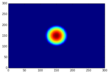
Dark Soliton Generation in Bose-Einstein Condensate using Phase Imprinting
This example simulates the evolution of a dark soliton in a Bose-Einstein Condensate. For a more detailed description, refer to this notebook.
from __future__ import print_function
import numpy as np
import trottersuzuki as ts
from matplotlib import pyplot as plt
grid = ts.Lattice2D(300, 50.) # # create a 2D lattice
potential = ts.HarmonicPotential(grid, 1., 1./np.sqrt(2.)) # create an harmonic potential
coupling = 1.2097e3
hamiltonian = ts.Hamiltonian(grid, potential, 1., coupling) # create the Hamiltonian
state = ts.GaussianState(grid, 0.05) # create the initial state
solver = ts.Solver(grid, state, hamiltonian, 1.e-4) # initialize the solver
solver.evolve(10000, True) # evolve the state towards the ground state
density = state.get_particle_density()
plt.pcolor(density) # plot the particle denisity
plt.show()
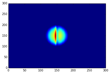
def dark_soliton(x,y): # define phase imprinting that will create the dark soliton
a = 1.98128
theta = 1.5*np.pi
return np.exp(1j* (theta * 0.5 * (1. + np.tanh(-a * x))))
state.imprint(dark_soliton) # phase imprinting
solver.evolve(1000) # perform a real time evolution
density = state.get_particle_density()
plt.pcolor(density) # plot the particle denisity
plt.show()
The results are the following plots:
Imaginary time evolution in a 1D lattice using radial coordinate
import matplotlib.pyplot as plt
import numpy as np
import trottersuzuki as ts

angular_momentum = 1 # quantum number
radius = 100 # Physical radius
dim = 50 # Lattice points
time_step = 1e-1
fontsize = 16

# Set up the system
grid = ts.Lattice1D(dim, radius, False, "cylindrical")

def const_state(r):
    return 1./np.sqrt(radius)

state = ts.State(grid, angular_momentum)
state.init_state(const_state)

def pot_func(r,z):
    return 0.

potential = ts.Potential(grid)
potential.init_potential(pot_func)

hamiltonian = ts.Hamiltonian(grid, potential)
solver = ts.Solver(grid, state, hamiltonian, time_step)

# Evolve the system
solver.evolve(30000, True)

# Compare the calculated wave functions with respect to the groundstate function
psi = np.sqrt(state.get_particle_density()[0])
psi = psi / np.linalg.norm(psi)

groundstate = ts.BesselState(grid, angular_momentum)
groundstate_psi = np.sqrt(groundstate.get_particle_density()[0])
groundstate_psi = groundstate_psi / np.linalg.norm(groundstate_psi)

# Plot wave functions
plt.plot(grid.get_x_axis(), psi, 'o')
plt.plot(grid.get_x_axis(), groundstate_psi)
plt.grid()
plt.xlim(0,radius)
plt.xlabel('r', fontsize = fontsize)
plt.ylabel(r'$\psi$', fontsize = fontsize)
plt.show()